


A Bit of Background Information
In 2003 I wrote a tutorial titled Expose Right. To my knowledge this was the first generally available essay that discussed the realities of digital exposure, as opposed to that required for film. Since then the technique described has become known as ETTR( E xpose T o T he R ight).
The main points of that essay, summarized and updated, are as follows…..
- A cameras sensor is an analogue device. When light hits a sensel (pixel) an analogue signal is generated. That signal is proportional to the amount of light received.
- Just for fun, it’s worth noting that film is essentially binary (digital) in nature. A grain of silver halide when exposed to light and subsequently developed turns black, or it doesn’t turn black, depending on various factors including, but not limited to, the amount of light that it receives along with the amount of development. It only is when a large number of silver particles are taken as a group that continuous tones are created, depending on how many grains are changed and how many aren’t in a given area.
- Just for fun, it’s worth noting that film is essentially binary (digital) in nature. A grain of silver halide when exposed to light and subsequently developed turns black, or it doesn’t turn black, depending on various factors including, but not limited to, the amount of light that it receives along with the amount of development. It only is when a large number of silver particles are taken as a group that continuous tones are created, depending on how many grains are changed and how many aren’t in a given area.
- This analogue voltage is then converted into digital format within the camera by an IC called an Analogue to Digital converter. This conversion is done in either 12, 14 or 16 bits, which has the ability to contain 4,098 (12 bit), 16,384 (14 bit) or up to 65,536 separate tonal values (16 bit).
- This digital data is then either saved to a data card as a proprietary raw file, or converted inside the camera into a JPG file.
- A JPG file is in 8 bit format, which means just 256 tonal values, regardless of what the bit depth of the camera may have been originally. A JPG is also in the sRGB colour space – much smaller than the camera is capable of recording – and also suffers lossy compression. (Now you know why photographers looking for high image quality never shoot JPG).
- A JPG file is in 8 bit format, which means just 256 tonal values, regardless of what the bit depth of the camera may have been originally. A JPG is also in the sRGB colour space – much smaller than the camera is capable of recording – and also suffers lossy compression. (Now you know why photographers looking for high image quality never shoot JPG).
- Most current DSLRs and digital backs have a dynamic range somewhere between 8 and 12 stops.
- Data in the raw file is linear. There has been no tone curve applied. This is done later in the raw processor.
- Film has a characteristic tone curve. The human eye sees logarithmically. But digital sensors are inherently linear. Double the light and twice the voltage is generated. This then ends up producing more or less twice the data.
- A typical consumer DSLR recording 12 bits per sensel is able to record up to 4,098 separate tonal values.
- If we assume a 10 stop dynamic range this is how this data is distributed…
- The brightest stop = 2048 tonal values
- The next brightest stop = 1024 tonal values
- The next brightest stop = 512 tonal values
- The next brightest stop = 256 tonal values
- The next brightest stop = 128 tonal values
- The next brightest stop = 64 tonal values
- The darkest stop = 32 tonal values
- As can be seen, each stop from the brightest to the darkest contains half of the data of the one preceding it.
- If we assume a 10 stop dynamic range this is how this data is distributed…
- This helps explain why noise is seen most in the darkest areas of a file. In the brightest areas there is a lot of data and so the noise floor (which is always present) only represents a small percentage of the total signal (or data). In the darker areas, where data is sparse, ever-present noise becomes easily visible.
So What?
OK. Maybe you knew some of this, or even all of it. But – so what? And why is this relevant to the statement made in this essay’s sub-title that camera makers are giving us 19th Century exposures, which are sub-optimal. Read on.
Black Cats and White Cats
Let’s imagine two cats. A black one and a white one. The black cat is sitting on a pile of coal and the white cat is sitting in a snow bank. You point your camera at the black cat on the pile of coal and take a picture. Now you point your camera at the white cat sitting on the snow bank and take a shot.
What do these look like? Unless you have compensated the exposure they will both look pretty much the same. The black cat and coal will look grey, and the white cat and snow will also look grey.
Why? Because, of course, light meters integrate the light that they see to produce an exposure centered on 18% gray. Zone 5, if you are familiar with the Zone system. This is about the same tonal value as concrete.
Take a picture of a typical scene, one with light tones, dark tones and medium tones, and a light meter or even the nifty 500 segment super-meter in your DSLR will do a pretty good job. But, present it with a gray card, a concrete sidewalk, a black cat on coal or a white cat on snow and the exposures set will all be about the same in appearance.
The Clever Photographer
But, of course we’re more clever than our dumb cameras. We understand this, and we know how to use our camera’s exposure compensation control. We know that we need to decrease our exposure a stop or two so that the cat and coal look truly black, and increase our exposure a stop or two so that the white cat and snow indeed look white.
Right? Well, yes, sort of. If you were shooting film, especially transparency film, this would absolutely be the right way to obtain the best exposure in each case.
But – Not For Digital!
In the case of the white cat and snow – yes – you would do the same as for film – increase the exposure so that it looked correct. But in the case of the black cat on the coal pile you would do the opposite of what you would do for film. Instead of decreasing the exposure to make the cat and coal look black, you would increase the exposurethe sameas you would for the white cat and the snow .
Why?
Well, there is the story of Willy Sutton the famous American bank robber. When he was finally arrested, he was ask, “Willy, why do you rob banks?” Willy answered, “Because that’s where they keep the money.”
The reason why we want to expose every shot that we take with the data as far to the right of the histogram as possible is becausethat’s where the data is! It also is where the visible noise isn’t. The visible noise is lurking in the darker stops.
There is actually more noise in the brighter stops, but because there is such a high signal level any noise is rendered invisible because of the superior S/N ratio.
A colleague measured his Canon 5D MKII and reported the following…
“My 5D Mark II has a noise level of ~70 units at its maximum highlight level of 16,383 (on a 14-bit scale), and a noise level of ~30 units at a much darker signal level of 16 (i.e., 10 stops darker). The highlights appear clean because the SNR is good (16,383 vs 70). The shadows appear gross because the SNR is dismal (16 vs 30) – in fact, the signal is buried in the noise.”
Some Caveats
Now, just to be sure that there is no misunderstanding – this approach only applies to raw files, not in-camera JPGs. Secondly, this means that you should bias your exposure towards the highlights, and the right side of the histogram.But, it definately doesn’t mean blowing the highlights.
And of course not every photographic situation will lend itself to this technique. A shot taken on a sunny day with a cloud, a mountain and a forest will challenge the dynamic range of any camera, and so there will be little opportunity of biasing the exposure toward the brighter tones without blowing out the clouds. There is no magic formula here. It’s simply the physics of sensors combined with good shooting practice.
Normalizing
Back to our cats. We take our two cat pictures (exposing both to the right) and then import these files into our favourite raw processing software. The white cat on the snow looks pretty good, and may require only minor adjstments. But the black cat on the coal pile looks totally wrong. Way to bright. What to do?
Easy. Just use the Exposure control (Lightroom and Photoshop / Camera Raw) or its equivalent in other programs, tonormalizethe image. In other words drag the whole range of data in the file from the right side of the histogram toward the left until it looks the way it should look and you want it to look.Voi la! A black cat.
A lot of extra work, you say. Why bother?
If you’ve been attentive, you’ll understand that by using this technique you have recorded the black cat and coal with many thousands of data values instead of just hundreds, which would have otherwise been the case. This means that you have a rich range of tonalities recorded which will make your photograph that much more interesting and attractive. But you will also have recorded with much less noise than if you had placed the cat and coal at the left of the histogram, which is where noise lurks.Normalizingthe image by moving the data from the right of the histogram to the left makes the tonal values look appropriate while at the same times avoids the noise that would otherwise be found in the lower quarter tones.
And that is what ETTR is all about.
Mark Dubovoy writes that the use of a camera’s auto-exposure can cause what he calls Tonality Suckout. You can read about this in his recent essay on Safari photography.
Welcome to the 21st Century
Regretably, this welcome does not include camera makers. They are still making all of their cameras, even the most expensive pro models, with 19th Century exposure techniques.
Since the introduction of CMOS sensor equipped cameras with Live View capability cameras have had the ability to analyse the image being shot in real time. That’s what your rear LCD histogram is all about in Live View. It is a real-time analysis of the image, displaying where on the tonal scale every pixel being captured is to be found.
This information could easily be used by the camera to automatically calculate and set the absolutely optimum exposure for any and every scene . This would be with the brightest (non-specular) part of the image placed just below clipping. The rest of the tonalities would then fall where they may, but would be most appropriately recorded, with the largest possible range of tonal values, widest possible dynamic range, and with the lowest possible noise.
A Custom Function that allowed the user to set the specular crossover point would be welcome.
One colleagure who I asked to review a draft of this essay wrote the following, which will be of interest to the more technically minded…
One possible UI for ETTR is a button press that sets the exposure. Similar to how a separate button on many cameras can be configured to perform autofocus. That provides a way to shoot many images with the same exposure, useful for situations where you want the exposure times to be the same.
There does need to be robustness in the system so that spurious hot pixels don’t fool the ETTR. A simple solution is allowing some small % of the brightest pixels to clip, somewhere between 0.01% and 1%. Possibly default to an auto-calculated %, and let an advanced user specify the desired %. To make it fast, perform a 4x or 8x downsample (level 2 or level 3 of an image pyramid) to work with fewer pixels.
Most of the noise in an image is just photon noise (shot noise) from the light itself. In a Poisson distribution, the variance (the square of the noise) is equal to the mean. So with each additional stop of light captured, the square of the noise doubles, which means the noise itself (the std dev) only goes up by a factor of sqrt (2). This is why SNR improves with more exposure (2x the light means only 1.4x the noise), which is why ETTR works. A simple but quite accurate noise model for digital capture is just a square root function:
noise (x) = sqrt (A*x + B)
where
x is the average signal (say, in a normalized range from [0,1])
A is determined by the size of the pixel and the chosen ISO (A*x is the photon noise), and
B is the noise floor of the sensor, which is independent of the # of photons you captured
With a perfect noise-free sensor, B is zero, but you still have A — darn it!
With no light (taking pictures of the black cat in a cave, or in my case, taking pictures with a lens cap on with the lights off), you have no photon noise since x is zero, but you still have B because sensors aren’t perfect — darn it!
As you can see, as x grows, so does noise (x). You can easily measure noise by taking a picture of a uniform area and measuring the mean and variance of the pixels. Do this for several exposure levels to determine a set of data points. They should lie on a straight line. The slope of that line is A, and the y-intercept of that line is B. Voila, the fundamental noise properties of your sensor!

Because the camera knows how much additional exposure is being applied above the usual “average” exposure, it would be trivial for it to generate a rear LCD preview that appeared “normal”, and similarly a simultaneous JPG could easily be produced that also looked “normal”. Indeed the entire process could be made invisible to the photographer, except that every shot taken would have about a half stop to three stops better dynamic range and consequently lower noise.
The raw file, as exported to a raw converter, would of course look overexposed. This could require the user to “normalize” the shot manually. But, not necessarily. Since the camera knows the delta between the technically optimum exposure and the one that the camera’s metering system deemed most “pleasing” it would again be trivial to encode a correction factor into the raw file which any raw processing program could subsequently read and then apply to normalize the image, even before the user saw it on-screen.
A colleague who is professionally involved in writing raw processing software for a major company provides the following comment…
“DNG has a tag named BaselineExposure that can be used for exactly this purpose. For example, if a camera captures an extra 1.5 stops above the auto-metered value, the camera should record a BaselineExposure tag value of -1.5. The raw processing software compensates by reducing the exposure of the recorded values by 1.5 stops from its default rendering of the image. Thus, the photographer reaps the benefit of ETTR and sees a sensible default rendering, without jumping through extra hoops.”
There is another important reason why auto-ETTR should be something that camera makers adopt. This has to do with white balance. Currently, there’s no easy way to tell whether an individual raw channel (i.e., BEFORE white balance) has actually clipped, which is what really matters for ETTR. The rear LCD histograms are currently based on already-rendered data (after white balance, color profiles, etc. have been applied).
For example, with a typical DSLR, when photographing a red flowers under natural daylight, the LCD histogram will typically show the red channel as blown out. This doesn’t tell whether the native raw red channel is actually blown. So one doesn’t know whether to increase the exposure for ETTR, or reduce it. The natural reaction of most users is to say, “Uh oh, I’m gonna blow the red channel in these flowers, so I better reduce the exposure till the red histogram doesn’t look blown out anymore.” Unfortunately, that’s almost always the wrong thing to do. In fact, the red channel (in the raw data) rarely clips on a typical DSLR with a normal daylight exposure, because the red sensitivity is very low (about 1.5 stops darker than green). If one was to reduce exposure till the red histogram no longer showed clipping, then the actual raw red channel would be very underexposed with a poor SNR. Result: noisy red flowers!
One colleague reports that he measured the relative sensitivity of the R, G and B of his DSLR at 5500K daylight (per daylight film). The ratio between the channels was very close to (G:B:R) 5:2:1. That helps explain the reasoning above. Food for thought.
If you think about it, the complex TTL metering systems that manufacturers have built into cameras for the past 60 years are all but obsolete. A live-view histogram-based auto-exposure system is all that needed to generate the best possible exposure from a technical perspective.
The Take-Away
So – here we are, more than a decade into the DSLR revolution (and the new century) and camera makers are still using 25, 50, even 100+ year old exposure technology in our latest cameras. Why? I really can’t say, but they should be taken to task for not delivering the best image quality that their cameras are capable of.
I have been advocating the ETTR approach to exposure since 2003, and have been discussing with colleagues how it might be automated within cameras since the first Live View capable cameras appeared about five years ago. I don’t think that there has been a conference, workshop, or seminar that I’ve been involved with for the past several years where this topic hasn’t been energetically discussed. Leading photographers, writers, educators and other imaging experts all seem to agree that auto-ETTR is something that’s long overdue from camera makers.
Yet, manufacturers don’t seem to have gotten the memo (or they’re ignore it for unfathomable reasons). Instead, our 2011 sensor-based cameras still have 1960 exposure technology. Maybe this essay can light a fire under some of the more forward-thinking camera makers to move from the film exposure paradigm of yesteryear to the realities and needs of 21st Century digital image capture.
Michael Reichmann
August, 2011
Note 1:
I would like to thank the group of colleagues who read and commented on an early draft of this essay. I have incorporated some of their suggestions, and even cribbed some text from their emails when their descriptions were better than what I could come up with. These are some of the brightest and most knowledgable professionals in the photographic and digital imaging field, and so if there are any errors in this essay they are almost certainly mine.
Note 2:
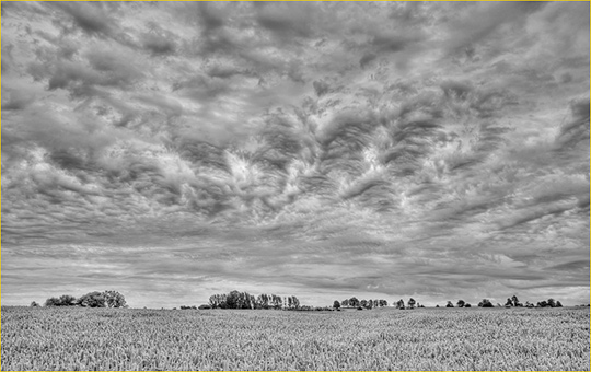
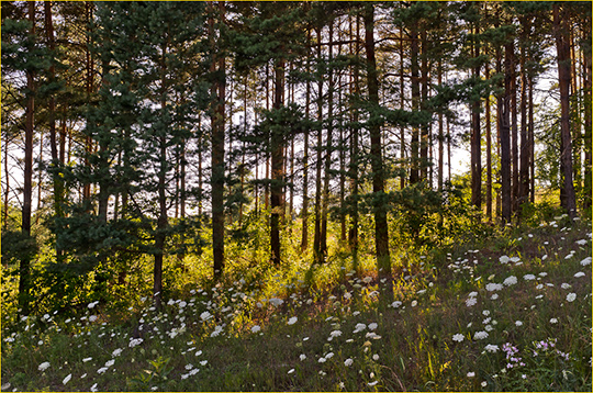
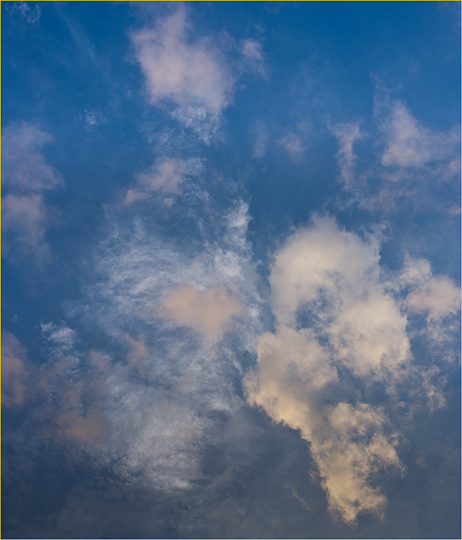
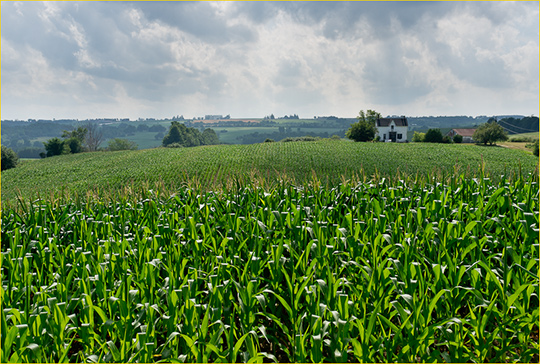
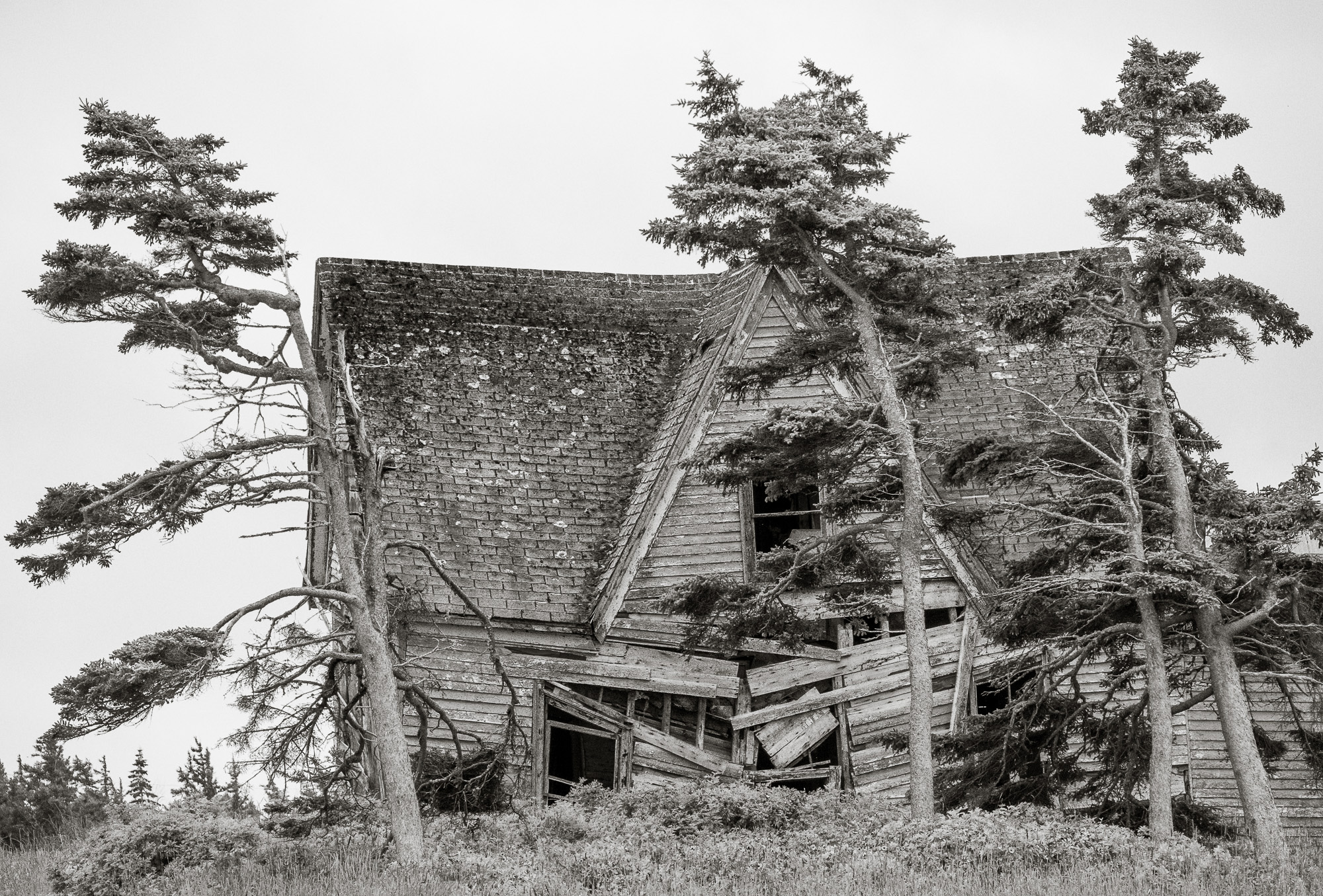
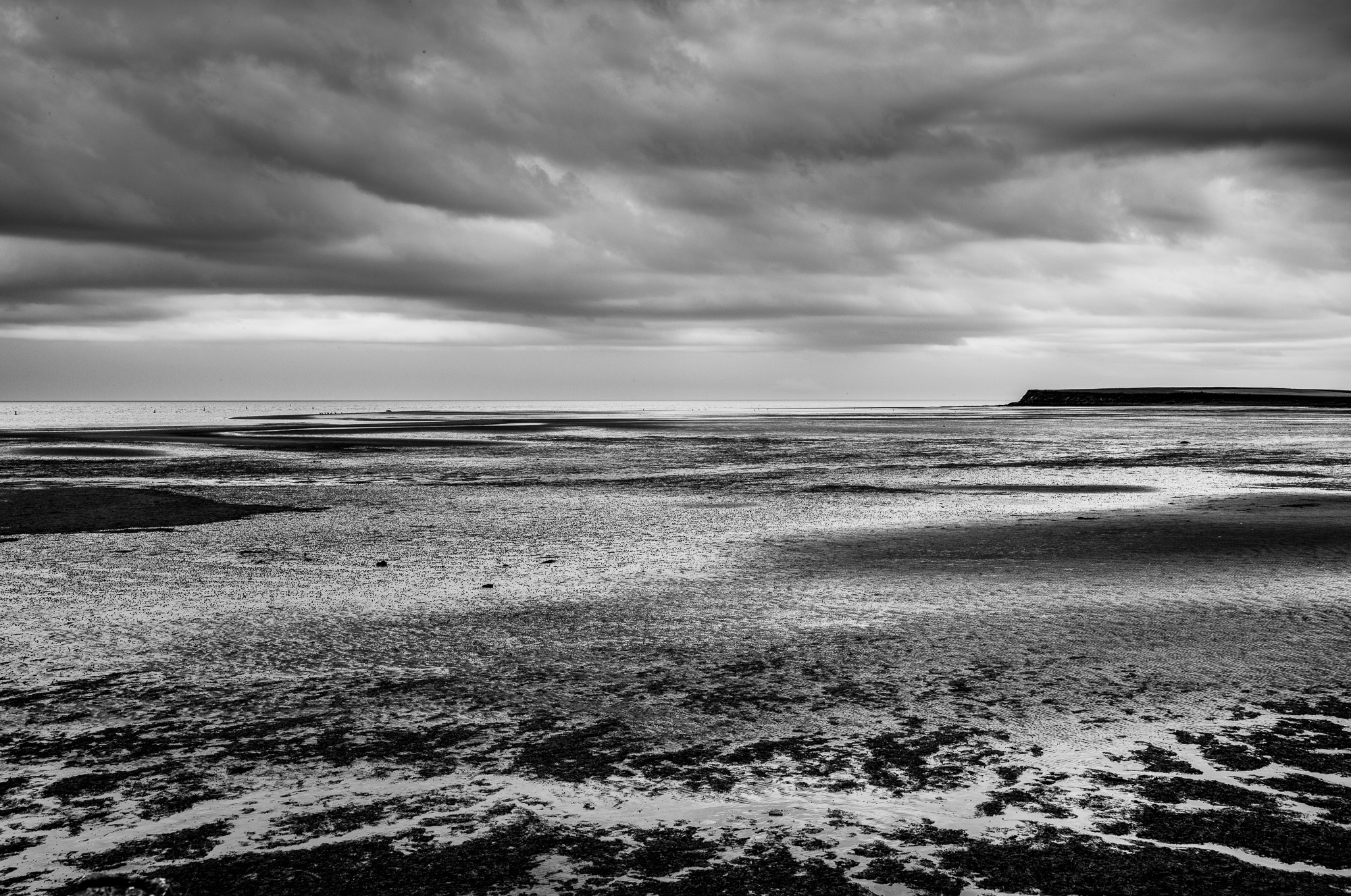
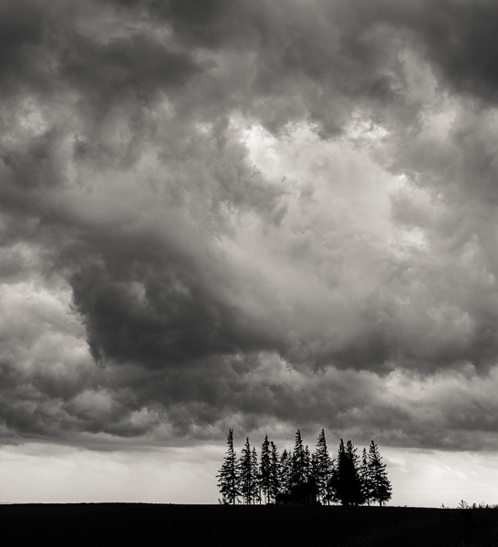
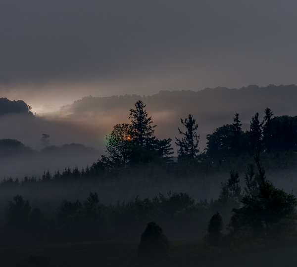
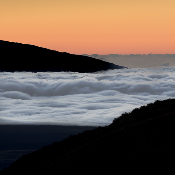
The photographs on this page were all taken with the highest level of ETTR possible. This allows for maximum dynamic range without the need for multiple exposures and HDR.
Note 3:
From a reader… “FYI, those of us in the industrial, raw processing business (factory automation and robotic vision), follow the ideas outlined in your article as standard practice. This includes auto ETTR followed by auto adjustment based on applying the negative of the exposure correction to produce ETTR “.
Updated: March 29,2015
Elevate Your Vision


Read this story and all the best stories on The Luminous Landscape
The author has made this story available to Luminous Landscape members only. Upgrade to get instant access to this story and other benefits available only to members.
Why choose us?
Luminous-Landscape is a membership site. Our website contains over 5300 articles on almost every topic, camera, lens and printer you can imagine. Our membership model is simple, just $2 a month ($24.00 USD a year). This $24 gains you access to a wealth of information including all our past and future video tutorials on such topics as Lightroom, Capture One, Printing, file management and dozens of interviews and travel videos.
- New Articles every few days
- All original content found nowhere else on the web
- No Pop Up Google Sense ads – Our advertisers are photo related
- Download/stream video to any device
- NEW videos monthly
- Top well-known photographer contributors
- Posts from industry leaders
- Speciality Photography Workshops
- Mobile device scalable
- Exclusive video interviews
- Special vendor offers for members
- Hands On Product reviews
- FREE – User Forum. One of the most read user forums on the internet
- Access to our community Buy and Sell pages; for members only.
You may also like