Noise, ISO and Dynamic Range Explained

This article examines the noise characteristics of a modern digital camera. The primary spec used to specify the noise performance of a camera is Dynamic range (DR). Most expositions on DR tend to get highly technical very quickly. OK, this article gets technical here too. However, I start with a heuristic approach to DR that doesn’t require any technical definitions, and (I believe) illuminates what DR means in a practical photographic sense. There are three primary noise sources in digital photography: photon noise, sensor nose, and analog-to-digital converter (ADC) distortion. I consider these in sequence, and at each step, we examine images of actual noise images. These are computer-generated noise images. The advantage of these computer simulations is that it allows me to isolate the effects of different noise sources. For example, with noise images from a real camera, it would be impossible to separate the photon noise from the sensor noise. The main conclusion developed here is that photon noise is by far the dominant noise in modern digital photography. Modern digital cameras have tremendous DR. Understanding that DR can inform our shooting techniques, such as ETTR (Exposure to the Right) and the use of auto-ISO. Hopefully, I have achieved the goal. As a bonus, I’ll explain dual-gain sensors.

A Heuristic Approach to Dynamic Range

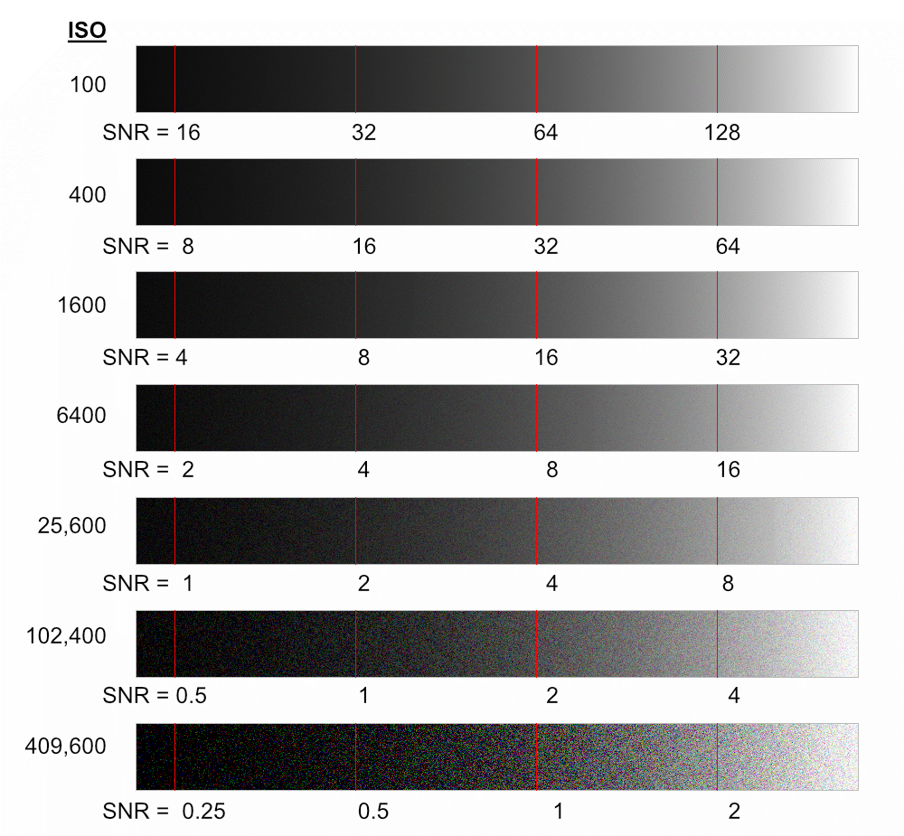
Let’s start by just looking at photon noise. Figure 1 shows seven noise gradients, each having an 8 stop range from full scale white on the right. Figure 1 is a computer-generated image. In the next section, I’ll provide more detail on how I generated these images, but for now, just accept that they are representative of noise in a modern digital camera, except at the highest ISOs. ISO is used here as the indicator of the noise level of each gradient. I’ll relate those noise levels to the photon counting of the sensor photodetectors in the next section. I use ISO as the general indicator of noise level because that’s what photographers use – not photon counts.

Start by looking at the virtually noise-free ISO = 100 gradient in Figure 1. Each gradient has an 8 stop range, but we see that the gradients fade to black at about -6 stops from full scale. I’ll call this 6 stop range the visual-DR because this is the DR range we can see. I am not suggesting that human vision has only about a 6 or 7 stop DR. A little discussion is required. Cone cells, the color detectors of the retina, saturate at about 100 photons. So cone cells have an (engineering) DR of log₂(100) = 6.5 stops. The human eye is highly adaptable, and it has a wide field-of-view. Yet the high-resolution part of the retina, the fovea, has only a 15 deg field-of-view.  The brain creates the perception of a scene. Fully a third of the human brain is devoted to image processing! As the eye darts around, it adapts. The iris can quickly adapt over a 4 stop range. The brain fuses scene fragments from the darting eye, much like an HDR merge, to produce our perception of a scene. Human vision is not like a camera. It is like a camera with powerful post-processing. If we include the fast adaptation of the darting eye, then one can realistically claim that the human visual system has 12 or 13 stops of DR. (Of course, we are not considering the 40 stops of slow adaptation from night to daylight vision.) My 6 stop visual-DR does not account for any adaptation, and for good reasons. Consider that perceived image created in the brain – what is its dynamic range? Just like processed HDR images, the perceived image is a compression of a wider DR observed across the scene fragments. Each fragment stops has 6.5 stops DR, and the adaptation (iris adjustment) occurs before the image fragments reach the brain. So we can only perceive an image with 6.5 stops DR, even if the “source material” was gathered from the scene has a wider DR. More important is that the end product of photography falls within this visual-DR. In my previous article, A Better Histogram, I showed that the histogram we see in our cameras and post-processing software only shows a 6-7 stop range. It may be worthwhile to review the El Malpais example in  A Better Histogram. Now, here is my alternative construction of DR. In Figure 1, pick the ISO level that you think provides minimally acceptable image quality across the visual-DR. This process uses our perception of noise, not an arbitrary SNR based definition. I believe most would agree that this minimally acceptable ISO (from Figure 1) is somewhere between 6400 and 25,600. ISO = 6400 is 6 stops above the base ISO = 100.  That means we can push the shadows in an ISO = 100 image up 6 stops and still have a noise level no worse than ISO = 6400. Let’s call that 6 stops the push–DR. Push DR is the range of image data that is “lost in the shadows” but is recoverable with a post-processing push. Then at base ISO DR = visual-DR + push-DR We’ll see that we lose one stop of DR per doubling of ISO, which is a reduction in push-DR. Take visual-DR to be 6 stops, and the acceptable image quality to be ISO = 6400, so the push-DR is 6 stops. Then DR = 6+6 = 12 stops. If we decide the visual-DR is 7 stops, or that ISO = 128,000 is the minimally acceptable quality level, then we get a DR = 13 stop. This is a subjective and arbitrary approach. However, you are about to see that the technical SNR approach to DR also is also quite arbitrary.

The SNR Approach

The definition of DR is the ratio of the strongest to the weakest signal level that the system can process, usually expressed using a logarithmic scale. I’m going to call these the “strongest” and “weakest” signal levels the top- and bottom-ends. Our logarithmic scale is the stop, or exposure value (EV) if you prefer. The Signal-to-Noise ratio (SNR) is the ratio of the signal level to the noise standard deviation. SNR defines the DR bottom-end as the signal level where the SNR falls below a threshold that defines minimally acceptable image quality. The definition most used by testing labs and camera marketing is the engineering DR, which defines acceptable image quality as SNR ≥ 1.  A less often used alternative is photographic DR.  Definitions vary, but here I’ll use SNR ≥ 10 for photographic DR. In Figure 1, I’ve indicated SNR levels under the noise gradients at points marked by the red vertical lines. SNR = 1 is pretty awful, but SNR > 8 appears to be pretty clean. So truth lies somewhere in between engineer and photographic DR. We have to take the threshold SNR approach with a big grain of salt. We’ll see that the difference between engineering and photographic SNR is embarrassing. Moreover, our perception of noise depends on the signal level. Look at the SNR = 4 across different gradients in Figure 1. SNR = 4 may be acceptable in the darker regions, but unacceptable in brighter regions of an image. In comparison, my visual/push-DR approach is that it defines “acceptable noise” based on our perception of noise across the entire visual-DR, not just at a single arbitrary SNR point. The advantage of the SNR approach is that it gives engineers a precise definition for doing measurements and calculations. Several modern cameras claim a DR of 15 stops. That’s engineering DR. When you read the fine print, you’ll find that these claims are for images that have been down-sized to 8 megapixels. That’s called print DR. Down-sizing is a smoothing operation that reduces noise, and hence, increases the DR figure. A 42-megapixel camera having a 15 stop engineering-print DR has engineering DR = 13.8 stops at full resolution.¹  That’s is not just marketing “specs-manship.” We need to use a print DR to compare cameras having different megapixel size. For example, according to DPReview, the Sony AR7 III (42 megapixels) and the A7 III (20 megapixels) have virtually identical print DR characteristics. Nonetheless, for the rest of this article, we’ll only consider full resolution DR. I’ll be using the Sony A7R III (my camera) as an example. The parameters that I attribute to the A7R III are from the NoiseProfile tag embedded in DNG files.^2,3

Photon Noise

The light signal is the illumination at the photodetector. Light is not a continuous flow. It comes in discrete packets of energy called photons. At a given illumination and exposure time, the actual count is a random variable. It has a mean count and a standard deviation. I denote the mean photon count using λ. Then λ = illumination x exposure time × photodetector surface area. For example, suppose λ = 2.5 photons. Then the most likely observed photon count values are 2 or 3 photons. We might also see 0, 1, or >= 4 photons, but with lower likelihoods. We take λ to be the signal level at the photodetector, as it is directly proportional to illumination.  Photon noise is the difference between the detected photon count and the mean value λ. The Poisson probability distribution governs the statistics of photon counting. We need only one fact about Poisson statistics: it has one parameter, λ. The mean count is λ, and the standard deviation is the square root λ^1/2. Photon noise is said to be signal-dependent because the noise level (= the standard deviation λ^1/2) depends on the signal level λ. The photon noise SNR is SNR = signal level / st. dev. = λ / λ^1/2 = λ^1/2 (photon noise only). As λ increases from dark to lighter regions of the image, the noise standard deviation also increases but only in proportion to the square root of the signal level. Thus, the SNR numerator wins the race, so SNR increases with the signal level but only as the square root of the signal level. SNR = λ^1/2 levels are indicated in Figure 1. The top-end of the sensor DR is the maximum number of photons it can count, which is called the Full Well Capacity (FWC). FWC is an important parameter that largely determines the sensor’s DR. The DNG NoiseProfile for the Sony A7R III indicates FWC = 48,500 photons.³ It is time to fill in the details of Figure 1. For each gradient, the “white-count” is the value of λ that corresponds to full-scale white. At base ISO, the white-count is the sensor’s FWC = 48,500 photons for the A7R III FWC.³  The successive ISO labels increase by a factor of 4 (= 2 stops), so the row white-counts are successively reduced by a factor of 4. For ISO = 100, 400, …, 409,600, the corresponding white counts are 48,500, 12,125, 3031, 758, 189, 47, and 12 photons. The “black-counts” on the left side (8 stops below the white-count) are 189, 47, 11.8, 2.96, 0.74, 0.19, and 0.05 photons. We can calculate DR of an ideal sensor that is degraded only by photon noise. The only sensor parameter we need is the FWC to define the top-end. The bottom-end is determined by the SNR threshold, which I’ll denote SNR₀ = 1 or 10 for engineering or photographic DR. Since SNR = λ^1/2, the threshold signal level is λ₀ = SNR₀² (again, for photon noise only). Then the photon noise DR is DR_photon = log₂( FWC/λ0 ) = log₂( FWC/SNR₀² ). No camera can avoid photon noise, so this is the theoretical limit of camera performance. For FWC = 48,500, SNR₀ = 1 yields engineering DR_photon = 15.5 stops, and SNR₀ = 10 yields photographic DR_photon= 9 stops. That’s a 6.5 stop difference between engineering and photographic DR! That’s just embarrassing. In the next section, we’ll add in the sensor’s noise, and that reduces this gap. Nonetheless, this huge gap is another indication of just how arbitrary the SNR based DR definition is.

Sensor Noise and Dynamic Range:

‘It’s the Photon Noise, Stupid!’

The two primary electronic noise sources in the sensor are the dark current in the photodetector and amplifier noise. The dark current produces false counts (due to thermal agitation rather than photons) that are indistinguishable from photon detections. Modern sensors have very low dark currents. However, it is cumulative. Dark current noise can be apparent in very long exposures as in astrophotography. Amplifier noise is also a thermal noise. Let σ_sensor denote the standard deviation of the sensor’s electronic noise as scaled to the photon level. (This does not mean that sensor noise is actual photons – just that we are using the photon level as a relative scale.) The Sony A7R III has a dual-gain sensor that has two base ISOs: 100 and 640. Two things change when the base ISO is switched: the FWC and the sensor noise level σ_sensor. In the low ISO state,100 ≤ ISO < 640, FWC = 48,500 and σ_sensor = 3.3 photons. In the high ISO state, FWC = 7,600 and σ_sensor = 1.01 photon. 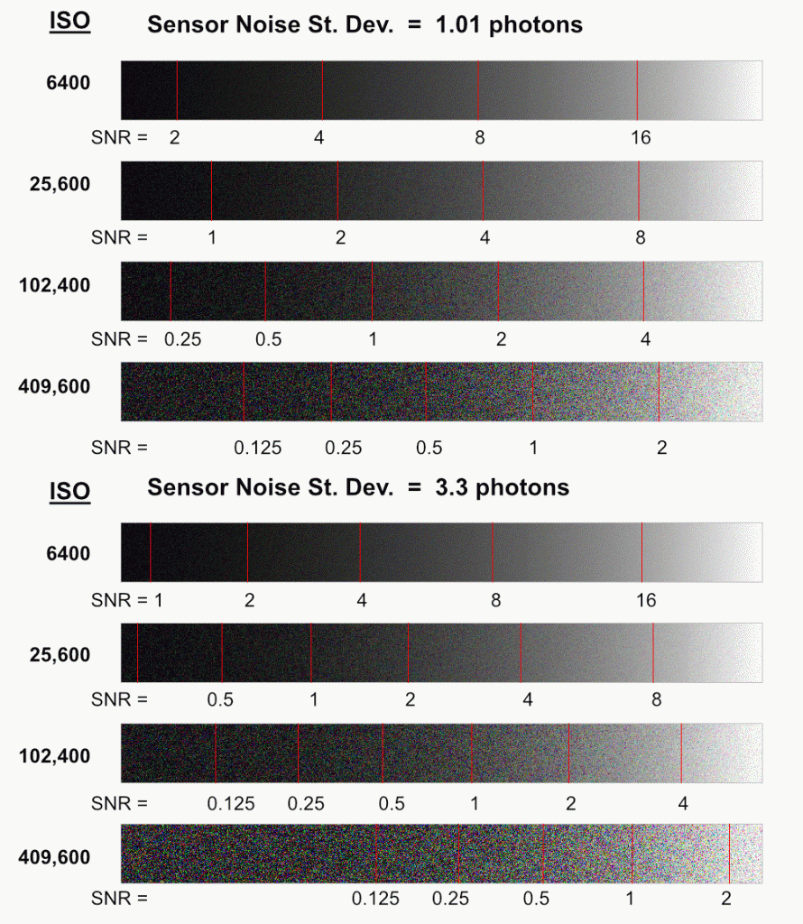Figure 2 is a rework of Figure 1 that shows both photon noise and sensor noise representative of an A7R III sensor. The ISO ≤ 6400 gradients are virtually identical to Figure 1 as photon noise dominates there. We see the effect of sensor noise (in the visual-DR) only at the higher ISOs.

While I’ve shown the sensor noise for both states of Sony’s dual gain sensor, keep in mind that only the low noise state, with σ_sensor = 1.01 photon, is used at high ISOs. There is more to the dual gain story – keep reading. Let’s consider what sensor noise does to DR. We have two SNRs: SNR_photon = λ^1/2 and SNR_electronic = λ/σ_sensor. The point where SNR_photon = SNR_electronic is λ^* = σ_sensor². For λ < λ^*, the sensor’s electronic noise dominates, and for λ > λ^*, it’s the photon noise. For the low ISO state of A7R III sensor, λ^* = σ_sensor² = 10.9. For engineering DR, the threshold photon noise only threshold λ₀ = 1 photon, which is well below λ^* = 10.9 photons. Thus, the sensor’s electronic noise limits engineering DR. Recall the photon only engineering DR is 15.5 stops, but for the A7R III electronic noise reduces this to 13.8 stops.⁴ For photographic DR, on the other hand, the photon noise threshold is λ₀ = SNR₀² = 100, substantially higher than λ* = 10.9 photons. Thus, the photographic DR is the same with or without the electronic noise: photographic DR = 9 stops. I’m repeating myself, but you can’t trust either of these numbers. Engineering DR is too generous, and photographic DR is too stingy. Reality falls somewhere in between.

The Role of ISO in Camera DR

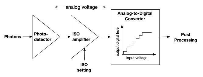
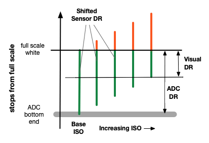
Next, we move beyond the photon level at the photodetector. Figure 3 illustrates the signal flow from the photon level to the digital domain. On the left is the photodetector that counts photons and converts that count to an analog voltage. At the other end is the analog-to-digital converter (ADC), which is the circuit that converts the analog voltage to a digital word. In between is the ISO amplifier. The ISO gain is proportional to the ISO setting.⁵

Figure 3 has two components that can limit DR: the photodetector, which we have discussed so far, and the ADC. Figure 4 illustrates how the ISO gain maps the sensor DR to the ADC DR to determine the overall DR at each ISO setting. The vertical axis is the signal level in stops. The amplifier is a multiplicative gain, but the logarithmic stops scale converts multiplication to addition. Thus, on the logarithmic stops scale, the ISO gain is a vertical shift of the sensor DR. Figure 4 shows how the ISO gain shifts the sensor DR levels to the ADC input range. The overall camera DR is the intersection of the shifted sensor DR and the ADC DR. Camera DR illustrated by the green bars in Figure 4. The orange part of the sensor’s DR is clipped at the ADC, and hence, not used.

The ISO on the far left is the base ISO, which is the ISO that maps the sensor top-end (= the FWC) to the ADC top-end. Increasing ISO from base ISO shifts sensor DR upwards, which reduces the camera DR (= the green bar). Since the ISO gain is proportional to ISO value, there is a DR reduction of one stop for each doubling in ISO.

ADC Dynamic Range

As illustrated in Figure 3, the ADC is a staircase response. That is a distortion, not a noise.⁶ So we have a problem. If it’s not a noise source, how do we calculate its bottom-end? There is a statistical approximation that models quantizer distortion as additive noise, but that relies on technical conditions that would apply only to highly textured images.⁷  However, we are more sensitive to noise in smooth regions, not the highly textured regions.  ADC impairment is most apparent as a banding effect on a smoothly varying image, not in highly textured regions. In my opinion, the “ADC as a noise source” model is just not applicable to photography. 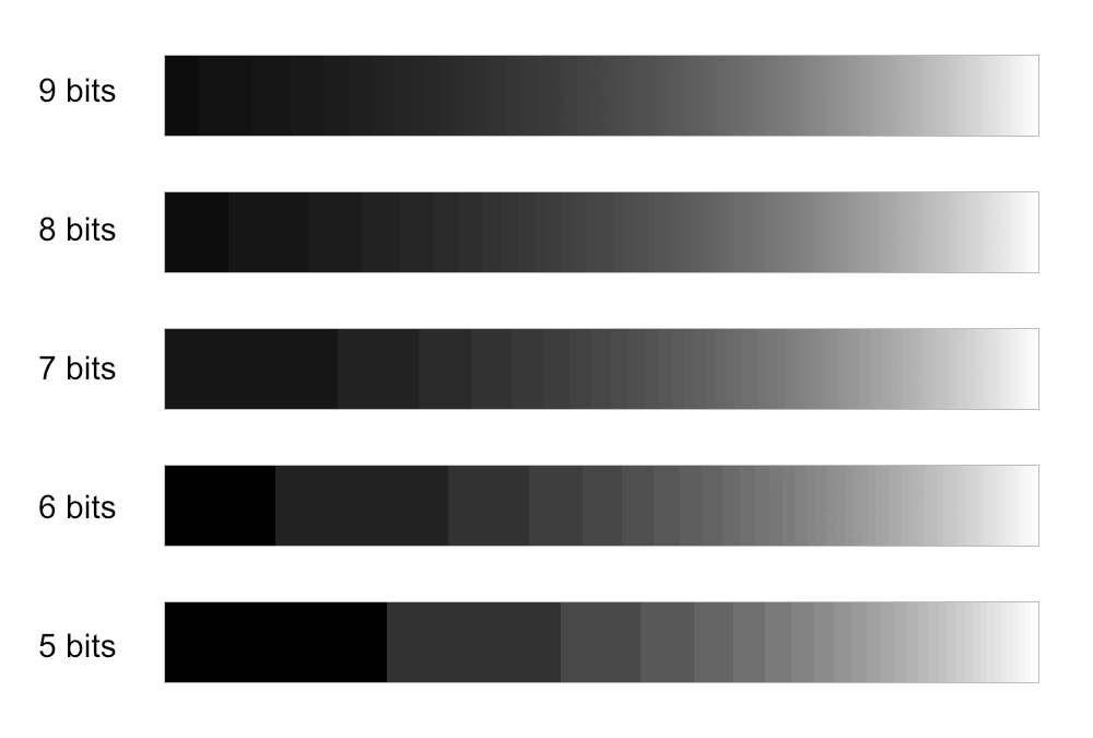Figure 5 illustrates ADC banding over 8 stops gradients. The quantization banding is evident at the lower bit widths. You can see banding at b = 8 bits, but it is faint.

A 1 stop gain (= a factor of 2 multiplication) applied in the digital domain is equivalent to a 1-bit “left shift” of the digital word. So, suppose we have a 14-bit ADC, and we agree that the visual-DR is 6 stops. Now apply a 6 stop push to the shadows. The banding observed in the pushed shadows is that of a 14-6 = 8 bit ADC, not the banding of a 14 bit ADC. So we can now apply my visual/push-DR method. In Figure 5, pick a bit-width that produces a minimally acceptable image quality. Call that b0. As before, it is subjective, but b0 = 7 or 8 bits seem reasonable. Then for a b-bit ADC, push-DR = b – b0 stops, which is the “left bit shift,” equivalently, the push gain in stops, that we can do and still have at least b0 bits of digital resolution. Thus, ADC DR = visual-DR + push-DR = 6 + b – b0. Thus, a 14-bits ADC has a 12 stop DR for b0 = 8. It’s 13 stops if we use b0 = 7. Hmmm, we’ve seen those numbers before. Note that this discussion of bit-width and dynamic does not apply to data stored in standard RGB formats (sRGB, Adobe RGB, etc.). Those file formats employ a nonlinear tone reproduction curve that improves quantization performance. That’s why we only need 8 bits for high-quality image storage, but that’s a different story that is not covered here.

Dual Gain Sensors

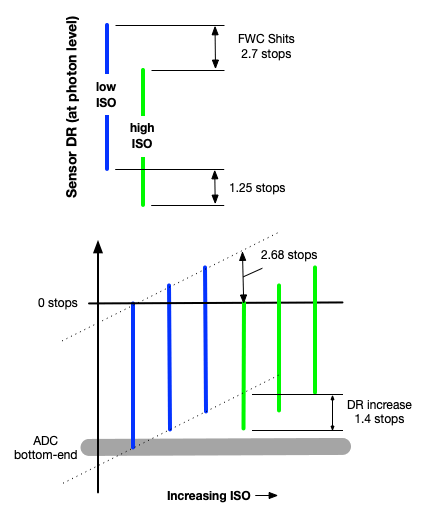
Finally, let’s revisit the dual gain senor. The dual gain sensor is a technology that was enabled by BSI (backside illumination) sensors.⁸ As previously noted, these sensors have two base ISO. The low base ISO has a larger FWC, but the sensor is noisier (larger σ_sensor). The larger FWC reduces base ISO and extends DR. We don’t need the inflated FWC for high ISO as that part of the sensor DR is now well above the ADC clipping level. Switching reduces the sensor noise, which significantly cleans up the higher ISOs, as we saw in Figure 2. The Sony A7R III has base ISOs are 100 and 640. For ISO < 640, FWC = 48,500 photons and σ_sensor = 3.3 photons. For ISI >= 640, FWC = 7,600 and σ_sensor = 1 photon. The shift in FWC is log₂( 48,500/7,600 ) = 2.7 stops. The shift in the bottom-end photon count is 1.25 stops due to the change σ_sensor. (I’ve omitted the math.) The upshot is that the low ISO sensor DR is 13.8 stops, while the high ISO sensor DR drops by 2.7 – 1.25 = 1.4 stops to DR = 12.2 stops. (These are engineering DR.) Figure 6 is Figure 4 redrawn for the A7R III dual gain sensor. The top figure shows the shift in sensor DR at the photon level. Observe that the sensor top-end maps to the ADC top-end at both base ISOs. Starting at base ISO = 100 with DR = 13.8 stops, we loose one stop of DR per doubling of ISO up to ISO = 640. With no switch in sensor state at ISO = 640, the DR would be 13.8 – 2.7 = 11.1 stops. However, notice that the 2.7 stop shift in FWC is the same as the shift in base ISO: log2( 640/100 ) =2.7 stops. So, switching the sensor state at ISO = 640 maps the high ISO FWC to the ADC top-end. With the state change at ISO = 640, we have DR = 12.2 stops at ISO = 640, an increase of 1.4 stops. Nicely done, Sony!

These last calculations are in engineering DR. For photographic DR, there is virtually no difference with and without the sensor noise. However, as noted above, it is the reduction in sensor noise (not the FWC) that opens up the higher ISOs. The low ISO boost in FWC reduces base ISO, and it relaxes design constraints on the photodetector that likely resulted in its incredibly low dark current. This is a really cool technology.

Conclusions

You’ve probably gathered that I don’t put much credence in the SNR approach to DR – certainly not down to fractions of a stop as reported in lab results. It is arbitrary, and it doesn’t relate to photographic practice. Nonetheless, it does facilitate precise measurements and calculations that provide a figure-of-merit for comparing different cameras. You can take my visual/push-DR to be simply a useful way to think about what DR means in photography. I do believe, however, that the visual/push-DR alternative could be formalized to a standard. That’s an issue for future debate. This information can inform us on how to use our cameras. I do landscape photography, and I spend a lot of time in post-processing. I shoot with my A7R III with ISO set to either 100 or 640, I adjust aperture and shutter speed manually, and I don’t use auto-ISO.⁹ I don’t worry much about underexposure because the DR is there to recover. I’m more concerned about blowing out cloud highlights than squeezing that last ETTR stop. That’s my style of shooting. It wouldn’t work for event photographers and photojournalists who need to get great shots out-of-the camera for rapid delivery to their clients. For them, auto-ISO, and aperture and shutter speed modes can be powerful tools. Hopefully, you can use this information to help you tweak the shooting style that is right for you.

Endnotes

1. Downsizing increases DR by log₂(N_FR/N_P)/2 stops where N_FR is the full resolution image size and N_P = 8 megapixels. 2. The DNG NoiseProfile specifies the total noise variance as Gx + O where x is the signal level normalized to the range 0 ≤ x ≤ 1. This model is used in post-processing algorithms such as noise reduction algorithms. It is described in the DNG specification, pages 67-68. O is the readout noise variance, which is dominated by the sensor’s electronic noise. G is the photon-to-normalized signal level gain; that is, x = Gλ. (The DNG spec uses S for scale factor, but I prefer G for gain.) Likewise, for ISOs above base ISO where we can assume ADC effects are negligible, the electronic noise variance of the sensor is σ_sensor² = O/G² photons². 3. FWC is deduced from the DNG noise profile as follows. x = Gλ, so the mean photon count corresponding to full-scale x = 1 is λ = 1/G. In particular, at base ISO, FWC = 1/G_base. I use base ISO = 100 because that’s what Sony says it is. Formally, FWC is the photon count where the photodetector saturates. The actual full-scale photon count is probably less than that extreme due to nonlinearity issues. I’m using the term FWC as the mean photon count for full-scale at the advertised base ISO of the camera, which likely less than the technically correct usage of the term. 4. We can calculate the actual threshold lambda for the combined noises. That requires solving a quadratic equation, which I’ll skip. The calculation does yield engineering DR = 13.8 stops. Or, we can just trust DPReview and DxOMark, which both report the same number. 5. Some cameras split the ISO gain between an analog gain and a digital gain to the right of the ADC. For our purposes, we suppose the ISO gain is purely analog. 6. As with all electronic circuits, the ADC does produce real noise. However, the primary degradation caused by quantization step distortion. 7. The ADC as noise approximation models quantizer error as additive noise that is uniformly-distributed on an interval of width being the ADC step size Δ. The noise variance for the uniform distribution is Δ²/12. There is information theory to justify this approximation, but it requires that adjacent signal samples be statistically independent. That translates to “highly textured” in images. Moreover, the noise approximation yields engineering DR = number of bits plus an extra 1.8 stops. If you believe that, let’s talk about a real estate deal. 8. The photodetector stores its photon count as electrical charge carriers (electron-hole pairs). The FWC of the sensor, which we’ve seen is the critical parameter that determines sensor DR, is increased by switching in extra capacitance. That extra capacitance consumes area on the sensor chip surface, which would reduce the area available for the photodiode. BSI provided the additional chip real estate needed for that capacitance behind the light-sensing side of the chip. Adding additional capacitance to the photodetector increases the FWC. That expands DR and reduces the base ISO. However, it also reduces the photons-to-photodetector voltage gain. In Figure 3, the total photon-to-ADC gain is split between the photodetector gain and the ISO amplifier gain. A reduced photodetector sensor gain must be offset by a higher ISO amplifier gain, which in turn increases the impact of the amplifier noise. The increase in DR by jacking up the FWC, however, is larger than the loss of DR due to amplifier noise. 9. It would be nice if I could program a button that would allow me to quickly switch between two ISOs, rather than having to futz with the thumbwheel.

---

John Sadowsky February 2020